Thanks to a sprinkling of Streamlit we now have an easy to use app for running your own simulations using our recently published model of the plant thylakoid membrane!

Here,  I’ll guide you step-by-step on how to run use the app.

Before we start, here are some Python packages you will need to have installed.

• Numpy

• Scipy

• NetworkX

• Streamlit

• Matplotlib

Running the simulations.

1. Download the code

All source code is available at

https://github.com/WhjWood/Thylakoid_Model

Go ahead and download the whole repository.

2. Launch the app

At the terminal, navigate to the folder with all the thylakoid_model source code

Then run the command

streamlit run Thylakoid_Model_App.py

This will prompt the app the pop up in the browser.

3. Set up the experiment

In the side bar, choose which experiment you want to simulate. Selecting “State I” or “State II” will parametrise the model with the same potentials we used in the manuscript.

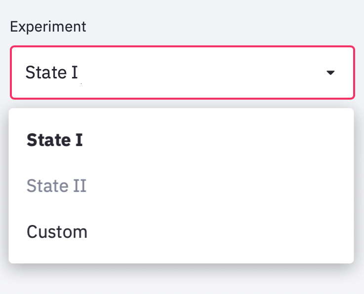
If you want to set up your own custom interaction energies for stacking, lateral and PSI-LHCII interactions select custom experiment (Here you can also choose between a 190 nm and 170 nm grana radius)

By default the post simulation analysis is not carried out and you will be left with a database of particle coordinates for each point in the simulation. 

It recommended that you tick “run post simulation analysis”. This will create a file in the output folder was statistics (such as percent of LHCII in grana, PSII average nearest neighbour distance etc)

Optional : You can run the chlorophyll network analysis by ticking “Run Network Analysis”.

4. Run the simulation

Once everything is set up you can run the simulation by clicking the button “Run Simulation”

The simulation will run in 3 stages:

• Equilibration – statistics must be sampled at equilibrium. For this reason 10 M Monte Carlo perturbations are taking ahead of the actual sampling. Progress will be be given in the terminal window

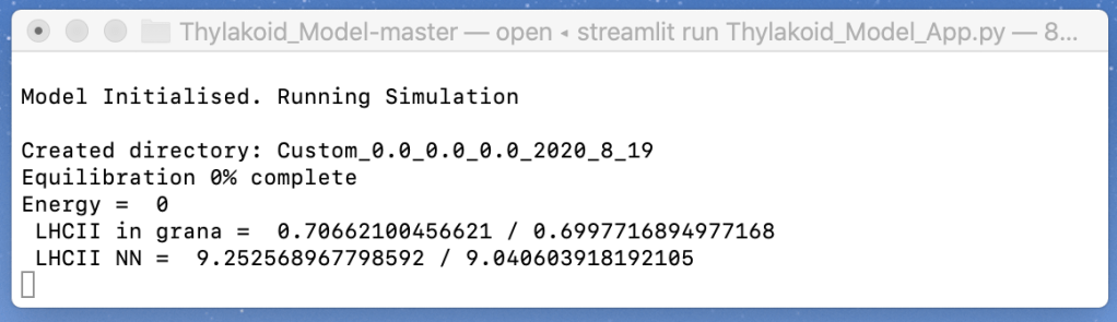
• Sampling. 1000 samples will be taken at equilibrium. During this stage, the terminal will display “Collecting Data”
• Post simulation analysis. The App window will show “Running Post-Simulation analysis

Finding the Data.

A folder will be created in the current directory to store the output

It will be called <Experiment>_<Grana Size>_<Potentials: Lateral, Stacking, PSI>_<date>

eg. “SI_190_2.0_4.0_0.0_20_08_20”

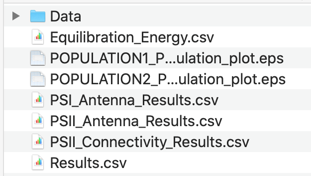
All post-simulation analysis results will be save in here. Standard analyses are saved as “Results.csv”. Network analyses are saved as “PSII_Antenna_results.csv”,”PSI_Antenna_results.csv” and “PSII_Conectivity_results.csv”. All analysis data will be save in CSV format with columns containing different variables and each row containing a sample. So to copy how I analysed the data in the paper, just take mean and standard deviations for each column!

Hamiltonian data at each Monte Carlo step is saved in “Equilibration_Energy.csv”. This is to be sure that equilibrium has been achieved.

Images of the two thylakoid layers will be saved as eps files and will look like this

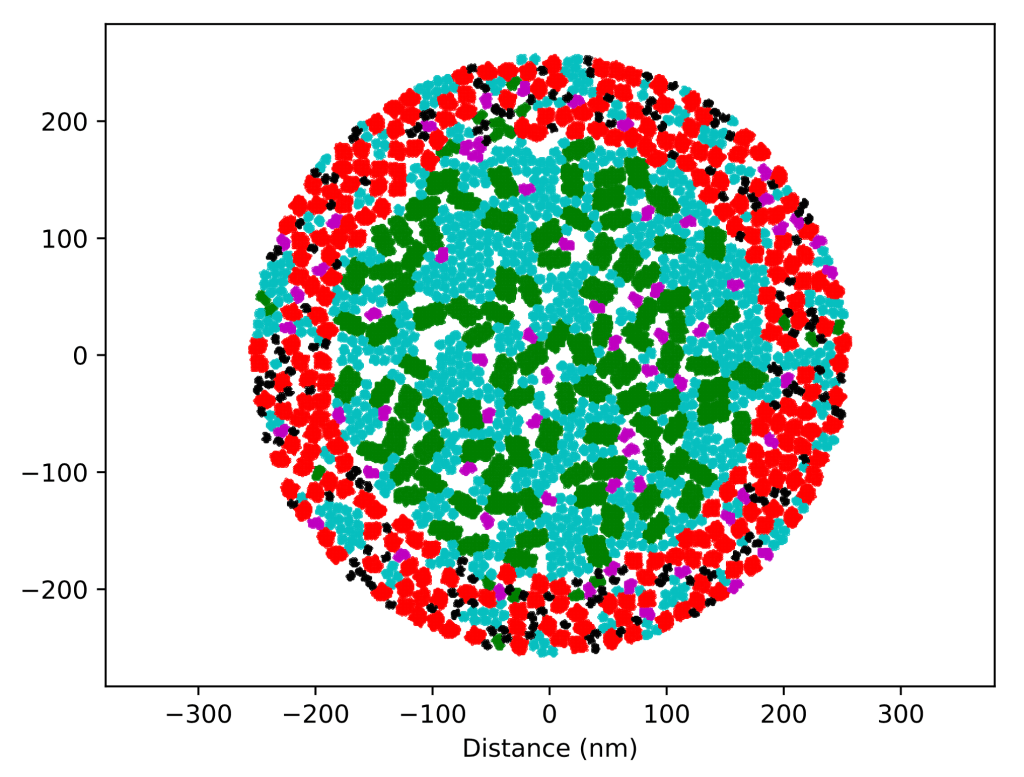
The raw particle coordinates will be saved in “Data” and called Population1… or Population2…

Files called checkpoints are from the equilibration stage so be sure to use those with numbers larger than 10 M (also note that Populations 1 and 2 refer to the two distinct thylakoid layers.